
How to use HLookup in Google Sheets is a common and burning question, as the function is not as famous as its counterpart VLookup. If you didn’t know this earlier, HLookup stands for Horizontal, and it functions similarly to VLookup. This function searches for the key value in the first row of the input range and returns the value of a specific cell from the column where it finds the key. Also, if it does not find the key, it will produce an error.
People who work with huge spreadsheets find themselves in dire need of finding a particular data in the haystack. Doing this manually can be time-consuming. However, like any problem, this too has a solution – HLookup. You can consider HLoop as the transposed version of VLookup – it searches horizontally instead of vertically. Thus, knowing how to use HLookup in Google Sheets is very important.
This guide will tell you how to use HLookup in Google Sheets and help you master the function.
Table of Content
| What is the Difference Between VLookup and HLookup? How Does HLookup Work? How to Use HLookup in Google Sheets – Syntax How to Use HLOOKUP in Google Sheets? Why Does HLOOKUP Doesn’t Work in Google Sheets? Can You Use VLOOKUP and HLOOKUP Together? Conclusion |
What is the Difference Between VLookup and HLookup?
There are many differences between VLookup and HLookup. Let us understand them one by one –

| Point of Difference | HLookup | VLookup |
| Definition | HLookup looks for the data horizontally in the table. | VLookup looks for the data vertically in the table. |
| Syntax | HLookup(lookup_value, table_array, col_index_num, [range_lookup]) | VLookup(lookup_value, table_array, col_index_num, [range_lookup]) |
| How it Works | HLookup assumes the data is arranged as a table with different elements of information in different rows. | VLookup assumes the data is arranged as a table with different elements of the information in different columns. |
| Usage | It is used to find out the data from a range in the bottom-most range. | It is used to find the data in the leftmost column. |
How Does HLookup Work?
The HLookup function in Google Sheets searches for a particular value in the first row of the table in the sheets. It returns a value in the column according to the index position by the formula parameter. The most important thing to note is – the lookup parameters have to be in the table’s first row. The HLookup function helps in finding both accurate and approximate matching.
HLookup focuses on looking up a value in a dataset and returning the value found in the spreadsheet table. Also, it is an inbuilt function in Google Sheets.
How to Use HLookup in Google Sheets – Syntax
The syntax for HLookup function is –
| =HLOOKUP(search_key, range, index, [is _sorted]) |
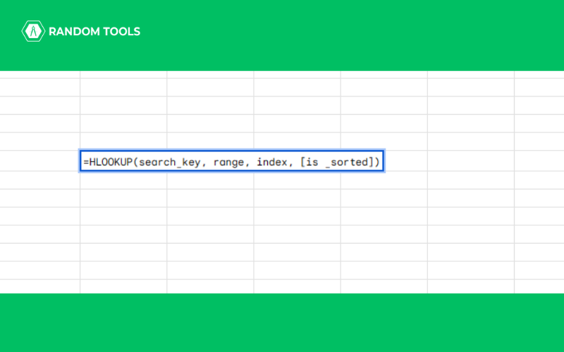
Here are the arguments for HLOOKUP –
- Search_Key – This is the value you search for. It can either be a numerical value or a string.
- Range – This argument defines the range in which the search_key will be looked up. Hence, the function searches for the first row for the key.
- Index – Theis arguments define the row index for the value to be returned. The first row in the range is numbered 1.
- Sorted – This is an optional parameter which is TRUE by default. This shows if the first row in the range is sorted in ascending or not, and if it is not, mark it as FALSE.
How to Use HLOOKUP in Google Sheets?
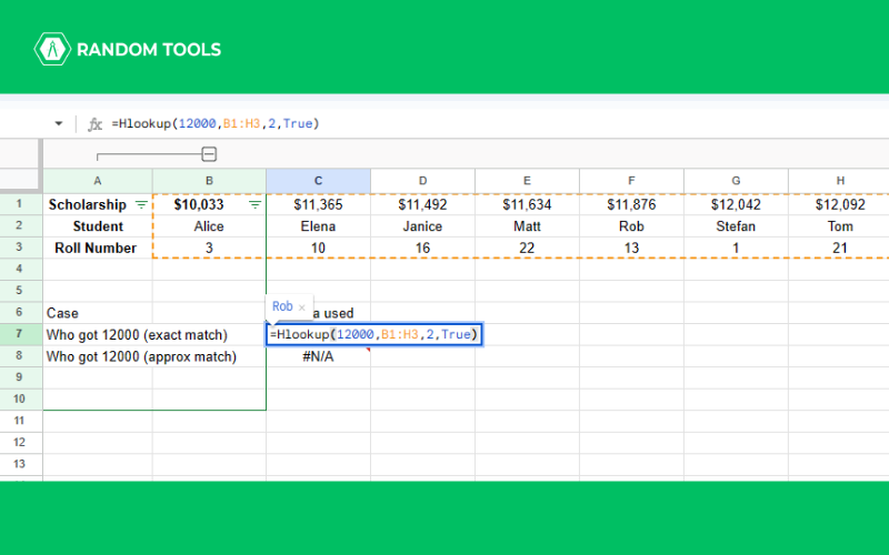
To start using HLOOKUP in Google Sheets, you need to have a set of data like the one given below. Here’s how to use HLOOKUP in Google Sheets –
- Click the cell to enter the formula.
- Start the formula with an equal sign (=).
- The first argument is the value you wish to look for in the data.
- Enter the cell range where the value will be searched for. Also, do not forget to enter a comma after inputting the cell addresses.
- Enter the third argument to define the row to show the corresponding value.
- Enter the final argument as FALSE. This is because the values are not in ascending order.
- Click Enter to execute the formula.
Now, to see which student got the highest marks, use the HLOOKUP function in tandem with the MAX function. In the MAX function, the cell address range is defined.
Why Does HLOOKUP Doesn’t Work in Google Sheets?
Sometimes, it might happen that HLOOKUP doesn’t work for you -it either gives you an error or does not give out the result. This is due to several reasons. Let’s discuss some of them below –
- The row from which you want to extract data is not present in the range you have chosen.
- The specified range does not include the row that should have a search_key, or it is not at the top of the list.
- The search_key is absent in the raw data, yet you enter FALSE in the HLOOKUP calculation.
- After entering a row or rows in the table containing the raw data, the formula’s index number is inaccurate.
- The raw data has many values that correspond to search_key. Usually, the formula simply returns the value of the first match and ignores any other matches. Therefore, you must ensure that there isn’t a duplicate row for search_key in the chosen “range.”
- There might be a typo in the search_key. So, it is advisable to avoid manual input to ensure errors are not happening.
Can You Use VLOOKUP and HLOOKUP Together?
Now you know how to use HLookup in Google Sheets, did you know it is possible to use VLOOKUP and HLOOKUP together. However, their formula patterns can be categorized into the HLOOKUP function in the VLOOKUP formula and VLOOKUP function in the HLOOKUP formula.
To combine the VLOOKUP and HLOOKUP, you need to tweak the data. Here’s how you can do it –
The HLOOKUP Function in the VLOOKUP Formula
First, here’s the syntax –
| =VLOOKUP(search_key, range, HLOOKUP(search_key, range, index, FALSE), FALSE) |
In the aforementioned example, we utilized HLOOKUP to locate the integer that serves as the index in the VLOOKUP calculation. It is better if the target row is the second row because HLOOKUP searches for data beneath the topmost column. The VLOOKUP function searches for the fifth column in the Lettuce row since HLOOKUP gives 5, which is in the second row in the April 2022 column inside the chosen region. This gives back 666.
The VLOOKUP Function in the HLOOKUP Function
The VLOOKUP formula functions as an index number finder for the HLOOKUP formula in this case, just like it did in the first formula. Because the VLOOKUP formula can search data starting from the leftmost column, you should add an extra column for the HLOOKUP index number adjacent to the Company column to the right as a precaution.
Given that the VLOOKUP function’s index number is 2, it returns 6 in the second column of the lettuce row. The HLOOKUP then identifies 666, present in the 6th row of the April 2022 column within the chosen field.
Conclusion
Now that you know how to use HLOOKUP in Google Sheets to find a specific value in the spreadsheet, you can efficiently work with large files and a pool of data. Google Sheets is one of the most used website applications people use in workplaces. It is easier to maintain, as users can edit and save changes in real-time.
Thus, how to use HLookup in Google Sheets is one of the basics of Google Sheets – learn to master the art of basic, and be a pro in your workplace.