
Your performance metrics, sales dashboards, app KPIs, decision-making, and other mission-critical activities are all compromised by duplicate data. Thus, you must know how to highlight duplicates in Google Sheets to ensure you have the right set of data instead of a bunch of duplicates that will hinder your efficient working.
In this article, we’ll detail each method for highlighting duplicates in Google Sheets and give examples.
Things to Keep in Mind Before Highlighting Duplicates
Try to make sure the following before attempting to highlight duplicates in Google Sheets:
- Remove any additional conditional formatting rules presently being used on your target cell.
- Make sure your searches don’t contain any blank spaces.
- When using Array Formulas to highlight duplication, avoid selecting headers.
- If possible, don’t highlight the provided duplicate values. Determine which cells the conditional formatting rule applies to. Next, select Trash from the Format>Conditional formatting menu.
Google, at times, does not recognize duplicates because of excessive space characters. This happens when one cell has leading or trailing spaces around the text but not the other. Since Sheets looks for a precise match, the extra spaces within the cells may cause overlooked duplicates. Using Google Sheets’ CLEAN features, you can get rid of excess gaps in your cells. You can avoid some hassles by taking care of these potential problems now.
Table of Content
| Things to Keep in Mind Before Highlighting Duplicates How to Highlight Duplicates in Google Sheets? How to Highlight Duplicates in Google Sheets – Single Column How to Highlight Duplicates in Google Sheets – Multiple Columns How to Highlight Duplicates in Google Sheets – Rows How to Highlight Duplicates in Google Sheets Using Added Criteria? How to Highlight Duplicates in Google Sheets Using the UNIQUE Function? Conclusion |
How to Highlight Duplicates in Google Sheets?
You can highlight the duplicates using conditional formatting and UNIQUE Function.
Conditional Formatting
The “Custom formula is” option in the conditional formatting rules is the most popular approach to highlight duplicates in Google Sheets. “Custom formula” enables us to use a formula to define which cells to format in accordance with a given criterion. For example, we may instruct Google Sheets to format values that are counted more than once.
How to Highlight Duplicates in Google Sheets – Single Column
You might indicate the range to which you want to apply conditional formatting in two ways. First, by choosing the range you wish to format before displaying the conditional formatting choice, Google Sheets will populate the cell range automatically. Second, the range to which you want to apply the formatting can also be entered in the “Apply to range” section of the “Conditional formatting” menu.
Here’s how to highlight duplicates in Google Sheets single column –
- The names in the dataset should first be selected (headers excluded).
- Select Conditional Formatting from the dropdown menu when you click Format in the top menu.
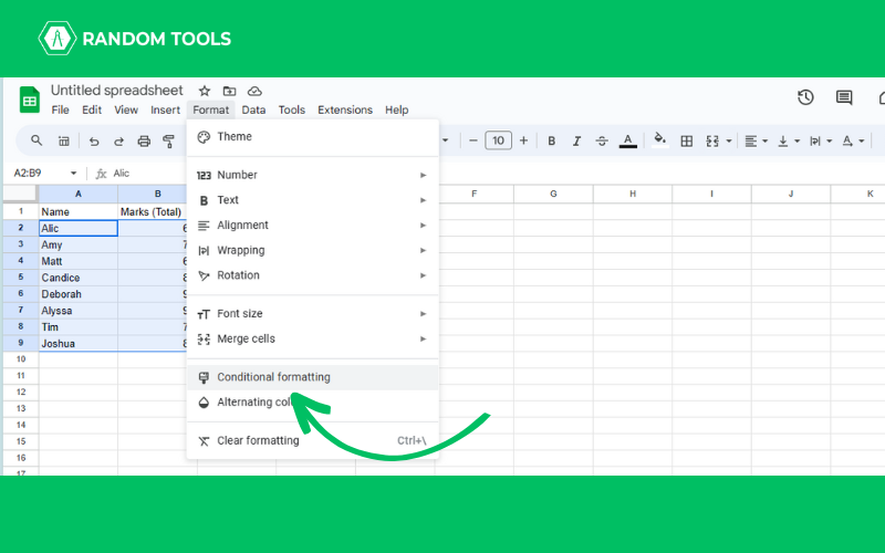
- On the side panel for Conditional format rules, click Add another rule.

- Click Format cells if... under Format rules, then choose Custom formula is from the drop-down menu.
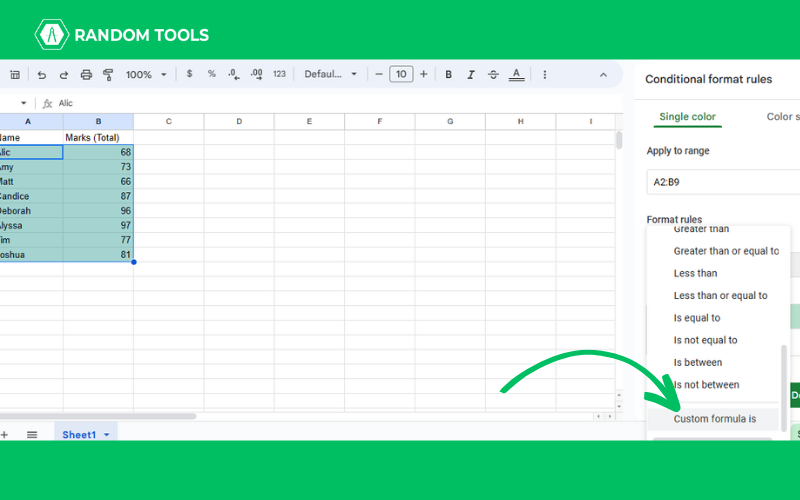
- Under the Format cells if… field, enter the COUNTIF formula.

- Then, by configuring the Formatting style choices, indicate how the duplicate cells should be formatted or appear on the spreadsheet.
- Select Done. The identical names will be highlighted using your chosen color and format in the column range.
You can remove the formatting without erasing the rule. Clear formatting can be selected from the dropdown menu after selecting a cell or group of cells and clicking Format on the top menu.
How to Highlight Duplicates in Google Sheets – Multiple Columns
Additionally, conditional formatting can be used to identify duplicates across different columns in a Google spreadsheet. Here’s how to highlight duplicates in Google Sheets in multiple columns –
- Select the data range, then choose Format > Conditional formatting.
- On the Conditional format rules side panel, click Add another rule.
- Double-check the cell range.
- Ensure all the columns you wish to look for duplicates are included.
- Select Custom formula by selecting the Format cells if… option.
- In the appropriate field, type the following formula.
- Choose the formatting style you prefer for highlighting duplicate data, then click Done. These three columns now show a spotlight on the duplicate names.
How to Highlight Duplicates in Google Sheets – Rows
You should follow the procedures outlined in the preceding example but make the following changes to the Custom formula:
- Choosing your data range without selecting the header row
- Select the Conditional formatting option and the Conditional format rules side panel from the Format top menu.
- Click Add another rule.
- From the Format rules option in the menu bar, choose Custom formula.
- Fill out the Value or formula field with the formula shown below: =COUNTIF(ARRAY FORMULA($A$2:$A$9&$B$2:$B$9)>1
- Select your desired color and formatting style for the highlighted duplicates.
- Select Done.
The following formula –
ARRAY FORMULA($A$2:$A$9&$B$2:$B$9) assembles the contents of each row’s cells into an array of strings. The ampersand is used to perform concatenation. The array is used in the COUNTIF formula. The condition looks like this: The condition is a concatenated string with all the values in a row.
$A3&$B3
The array is just a construct of the column type. The array’s combined string is checked for repetitions using the COUNTIF method.
How to Highlight Duplicates in Google Sheets Using Added Criteria?
To identify duplicate data, Google Sheets offers additional criteria. For instance, you may set your Sheet up to only show duplicates for certain values. Here’s how to highlight duplicates in Google Sheets using added criteria –
The star operator (“*”) is required in your syntax to instruct the COUNTIF function to consider both factors. The whole syntax will be as follows:
=(COUNTIF(Range,Criteria)>1)*(New Condition))
How to Highlight Duplicates in Google Sheets Using the UNIQUE Function?
A cell range’s unique values can all be found using the UNIQUE formula. A smaller dataset is ideal for the function. Here’s how to highlight duplicates in Google Sheets using the UNIQUE Function –
Simple syntax is used: =UNIQUE(Range)
Let’s use the same dataset for this function’s application to identify distinct values.
- Choose a blank cell.
- Enter the data range you want to check for unique data with =UNIQUE.
- The formula will return the unique values inside the range.
By removing complex formula setups, UNIQUE gives you a clean dataset free of duplicates. However, this function may have drawbacks in more complex duplication usage scenarios.
Conclusion
Your measurements, reporting, analysis, and decision-making are all impacted by the data in your spreadsheet. Duplicates are simple to identify and remove with Google Sheets, enhancing the data quality for your company’s operations. The techniques described in this blog post are easy but efficient approaches to guarantee improved data. Also, if you want to learn more about Google Sheets basics, visit here!