You must have felt really frustrated while hovering through the pile of data on a sheet. But, a simple function called VLOOKUP can help access your desired data. You have definitely heard of VLOOKUP in Excel, but here, we will learn how to use VLOOKUP in Google Sheets!
VLOOKUP is a powerful tool that helps you search through the data in a huge Google Sheet. No matter if you are a business owner or an employee of an organization, learning VLOOKUP can help you in many ways – it can help save you time, thus helping you make informed decisions. In this guide, we have discussed the major why you must use VLOOKUP and also how to use VLOOKUP in Google Sheets!
Table of Content
| How to Use VLookup in Google Sheets – What Does it Do How to Use VLookup in Google Sheets – Advantages How to Use VLOOKUP in Google Sheets? How to Use VLookup in Google Sheets – Best Practices Conclusion |
How to Use VLookup in Google Sheets – What Does it Do
VLOOKUP is a function that searches for a specific value in the leftmost column of a table of range and returns a corresponding value from a specified column within that range. Here’s the syntax of VLOOKUP –
| Vlookup(search_key, range, index, [is_sorted]) |
Here’s what each parameter does –
- search_key – It is the value that you want to search for.
- range – It is the table or range that you want to search in.
- index – It is the column number (starting from 1 of the value you want to retrieve)
- is_sorted – This input is optional, indicating whether the range’s data are arranged in ascending order. If the argument is set to TRUE or omitted, the function assumes the data is sorted and will use a faster search algorithm. The function utilizes a slower search technique that works for unsorted data if the argument is set to FALSE, though.
We can use an example to understand this –
If you have a table with a list of student names in the first column and their corresponding marks in the second column, you can use the VLOOKUP function to look up the price of a specific product based on the name. Now, without further discussions, let’s see why and how to use VLOOKUP in Google Sheets!
How to Use VLookup in Google Sheets – Advantages
VLOOKUP is an effective and easiest way to find something in a huge pile of data on a sheet. Here are some added benefits of using VLOOKUP in Google Sheets –
- Save and Time – This function automates the search. Thus making the entire process easy and convenient. This saves time and effort as compared to searching manually.
- Limited Error – If you search for something manually, there is a huge risk of making mistakes, such as misreading and mistyping the information or data. It can help you avoid these mistakes by performing an accurate search.
- Improves Data Analysis – VLOOKUP can analyze data more efficiently to compare and retrieve data from different tables. This can help you identify trends, patterns, and relationships between the data points.
- Increase Accuracy – VLOOKUP retrieves the correct information and data by avoiding incorrect or irrelevant information.
- Offers Customization – VLOOKUP allows you to customize the search specification and choose the column from which data needs to be retrieved.
How to Use VLOOKUP in Google Sheets?
It’s easy! Here’s how to use VLOOKUP in Google Sheets –
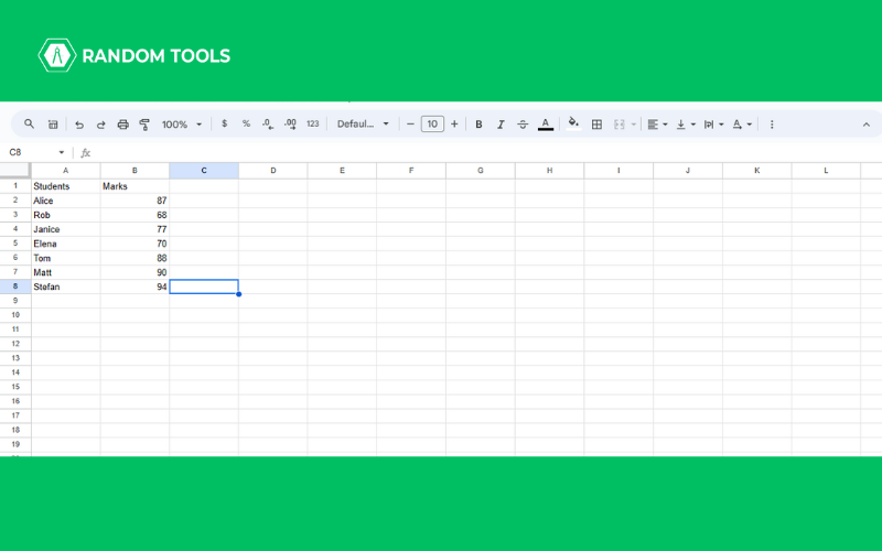
- Open a Google Sheet (new or existing).
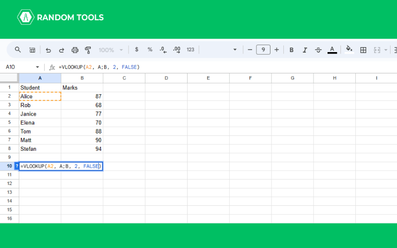
- Enter the data in column A as the students’ name.
- Enter the data in column B as the students’ marks.
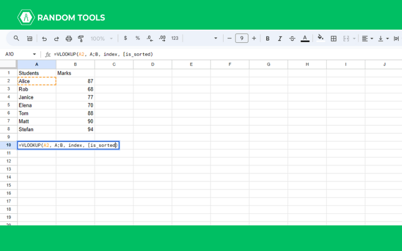
- Decide the column where you want to enter the function. You can pick any!
- Enter the formula into the selected cell. (=VLOOKUP(search_key, range, index, [is-sorted])).

- Replace the search_key argument with a reference to the cell containing the value you want to search for. Ex – If you want to search the marks of Alice, and if Alice is in cell A2, write A1 in the place of search_key.
- Now, replace the range argument with a reference to the range of cells that contains the data you want to search in. Ex – If your product names are in column A and your prices are in column B, you will replace range with A:B.
- If you are working with smaller data, you can click and drag your mouse over the cell range the VLOOKUP should use to retrieve the data.
- Now, replace the index argument with the number of columns containing the data you want to retrieve. Ex – If you want to retrieve prices from column B, you would replace index with 2.
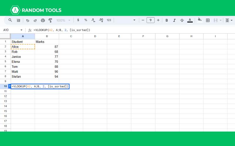
- In the final argument, if the data is sorted in ascending order, you can set it to TRUE or omit the argument completely. However, if your data is not sorted, you should set the argument to FALSE to ensure accurate results.
- Please Enter to apply the formula.

That’s it! You have your result. You can copy the formula to other cells in the sheet to retrieve the data.
How to Use VLookup in Google Sheets – Best Practices
Once you know how to use VLOOKUP in Google Sheets, there a few key points to remember before using VLOOKUP in the Google Sheets to ensure it works accurately –
Ensure the Data is in the Same Row
Ensuring the data is in the same row helps search the value accurately. If the data is not in the same row, VLOOKUP won’t be able to find the data.
Sort the First Column by Ascending Order
Ensuring the first column is in ascending order yields the correct data you are looking for. So, if you see the data is not sorted in ascending order, use the FALSE argument in the formula, and you will have your data.
Include Headers in the Formula
Including the header will tell the formula to know where to find the relevant data. Otherwise, the function could retrieve false or incorrect data. Ex – If you have column headers in Row 1, such as Students Name, Class, Marks – ensure these are also included in the range section of the formula.
Use Wildcard Character
Wild character (*) can be used in the lookup value to represent the combination of characters. Here’s how your wildcard character in the Google Sheet VLOOKUP formula will look like –
| =VLOOKUP(“Alice*”, A2:B10, 2, FALSE) |
In case of huge data, if there are multiple matches, it will retrieve the first one it matches.
Match the Formula to the Case of the Data You Are Looking
Like all the formulas, VLOOKUP is also case-sensitive. So ensure to enter the value in the same manner as you have entered in the cells. For example – if you have entered Alice in the cell and alice in the formula – it will give out an error.
Conclusion
VLOOKUP function really comes in handy if you are dealing with large files in the Google Sheet. Now that you know how to use Vlookup in Google Sheets, you can easily apply the formula and search for the desired result. The formula is somewhat like HLOOKUP!
Maybe it won’t work at the first go – but practice is the key to learning and uncovering skills. Also, mastering Google Sheets can help you know more about the formula. Thus, making you an amazing troubleshooter!