How to Make a Table in Google Sheets in 2023?

Tables are fundamental components of a spreadsheet that allow you to structure and complete data in one place. Though the basic concept of a table is the same, the basic varies depending upon the software you are using. This is why while using Google Sheets, you might sometimes have questions like – how to make a table in Google Sheets.

Excel and Google Sheets are similar, with a hint of differences that might cause the users to wonder. So, in this blog, we discuss how to make a table in Google Sheets and learn how to format it, which will help them be identified as tables. 

How to Create a Table in Google Sheets?

Like Excel, Google Sheets does not allow you to create a table. Instead, you can use borders and formatting to make a table. Creating a table is a two-step task. First, you need to open a spreadsheet in your browser. Once done, follow the steps below to create a table –

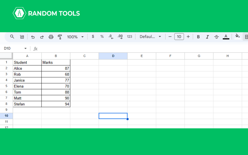
• Once you have your spreadsheet open, you can first enter the details that you want (like the ones mentioned below). 

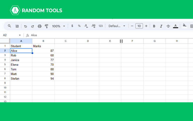
• You have your table ready. Now is the time to format and make it look more appealing and user-friendly.

Now that you know how to make a data table in Google Sheets let’s see how to make other tables and format them – to make them look more appealing and scannable. 

How to Make a Table in Google Sheets – Pivot Table

A pivot table is a semi-automated tool that presents custom summarization of large data sets to ensure you and other users understand it well. Without a pivot table, you might have to use several formulas and techniques that might seem cumbersome at times. Here’s how to make a pivot table in Google Sheets –

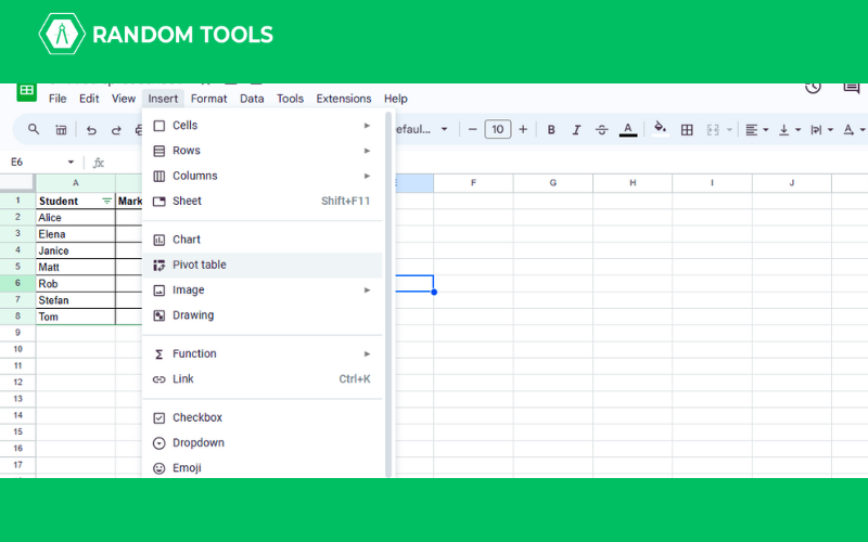
• Go to the Insert option in the menu bar and select Pivot. 

• Add a data range.

• If you want to insert the pivot table in the existing sheet, click the existing sheet. 
• Once done, click Create. 
• On the contrary, if you want to add the table to a new sheet, click on New Sheet. 
• Voila! You have a new sheet with a pivot table. 

A pivot table is also helpful if you have a question – how to make a frequency table in Google Sheets.

How to Make a Table in Google Sheets – Table Chart

Creating a chart or graph helps in sorting your data. Thus making it easier for you to read and understand. Here’s how to make a table chart in Google Sheets –

• Select the data you want to use. 
• Go to Insert. 
• Select Chart. 

• There will be a default bar graph just like the one below.

• There will be options to make a bar chart, pie chart, column, and line chart. 

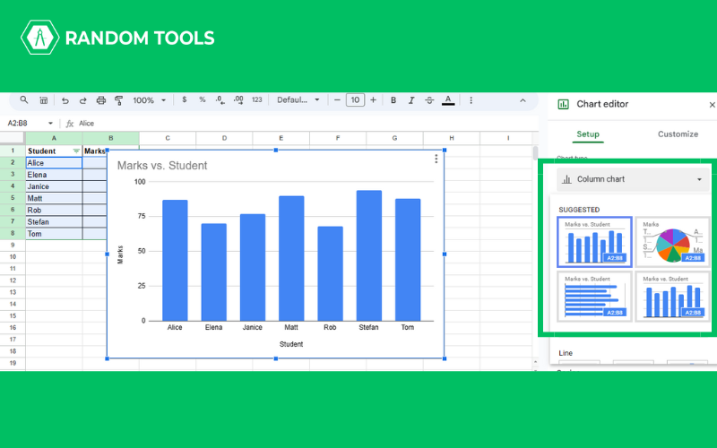
• Choose the chart type you want to use. 
• The chart updates automatically with the data given in the sheet. Also, you can customize any data or graph you want from the options at the side of the page.

How to Make a Table in Google Sheets – Border

Borders make huge differences in making your table look like a proper table. Here’s how you can do it –

• Once you have entered all the necessary details in the row and column, press CTRL+A to select the entire page.
• From the bar above, click the icon that looks like a border.

• You can select the type of border you want. In addition, you can also change the color of the border.
• Once done, your table will be something like this. 

How to Make a Table in Google Sheets – Formatting

Now that you have a table base ready, it is time to make it prettier, collapsible, filtered, searchable, and functional. Before that, you must know that there are no table formatting shortcuts. But here’s how you can format your table so that you can customize it according to your wish –

Apply Alternating Row Color

Here’s how to apply alternate row color – 

• Select the range of cells that contains your table, including the header. 
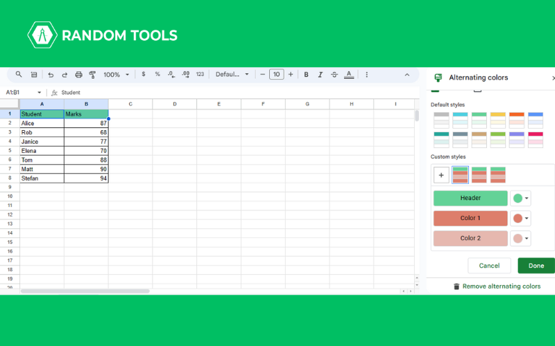
• Click on Format. You will see an option of Alternating Colors. 

• A page will appear at the side of the sheet, where you can see a green checkbox. 

• This happens when the Google Sheet will automatically recognize the headers. 
• If it is not checkmarked, you can do it manually. 
• In addition, you can also create a custom format by manually selecting the header color and the alternating color for the row. 
• Moreover, you can choose any one of the Google Sheets default to create a style of your own. 

• You can play around with the table formatting and select one that resonates with your brand or choice. 
• Once you are satisfied with the color, click on Done. 
• If you want to remove the alternating colors, click on Remove Alternating Colors below the end of the page.  

How to Make a Table in Google Sheets – Filtered Table

You must first know that Google Sheets allows one filtered table per sheet. However, you can use different tabs in one sheet. The filtering table helps you add filters to each column, allowing you to sort your data with a few clicks. Now that you know how it works, read below to create a filtered table –

• Select any header in your sheet. 
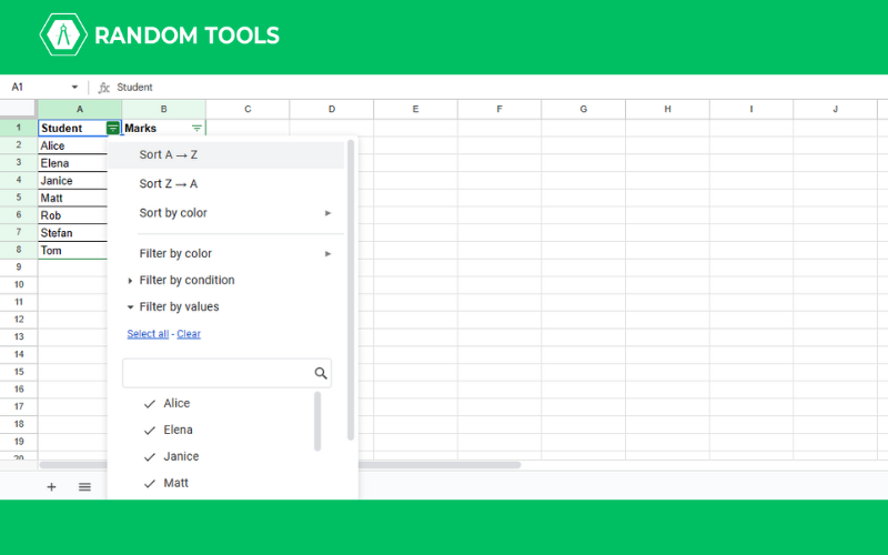
• Click on Data, and select Filter. 

• Click on the filter icon, as shown below, and you will find options for filtering and sorting. 

How to Make a Table in Google Sheets – Collapsible Table

Working with a large table can be annoying and frustrating at the same time. So, making the table collapsible can help you manage huge tables and also help you avoid mistakes. You can group the rows and columns to make your table collapsible. 

Here’s how you can group the rows in the table –

• Select all rows, but exclude the header. 

• Right-click on the row, select View More Row Actions, and select the option to group rows. 

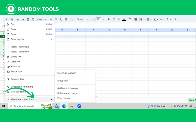
• On the top-left corner of the page, you will find a minus button.

• Click on the minus icon to collapse the rows. Also, to expand the row, click on the plus icon on the same left corner. 

Here’s how you can group the columns in the table –

• Select all the columns, but leave the header. 
• Right-click on the columns, select View More Column Actions and select the group option. 

• To collapse the table, click on the minus icon on the top left corner of the page.
• To expand the table, click on the plus icon on the top left corner of the page. 

How to Make a Table in Google Sheets – Searchable Table

A searchable and scannable table looks professional. The best way to make the table searchable is by naming the entire range. Also, you can name an individual column. This helps you to search the data you are looking for – all you need to do is search for the data using the name. 

Here’s how you can name your entire table and a specific column within the table – 

• Select the range of cells containing your table. 
• Click on Data and select Named Ranges. 

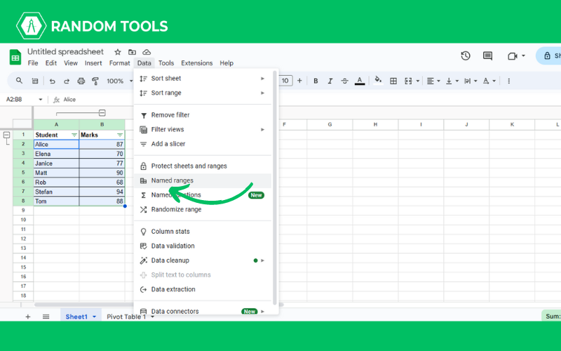
• Type in the name for the table, and click Done. 

• The table now appears in the Named Ranges sidebar. 
• Now, to add a name to your column in the table, select the column and click Add a Range. 

Naming a column helps you to reference it from other cells. For example, if you want to know the total marks, type the SUM function in an empty cell, and after parentheses, type the name of the column, and you will see a suggestion as given below. You can select it with the cursor or hit the enter key to select the column. Now, close the parentheses and hit the enter button. You have the sum of all marks. 

How to Make a Table in Google Sheets – Resizing Rows and Columns

You can resize your rows and columns in your Google to fit in your data. Here’s how to resize the rows and columns –

• To resize the column, click on the column header and put your cursor on the lies between the column header. 
• Hold and drag as per your desired size.

• To resize the row, click on the row header. 

• Place the cursor on the line between the row header and drag to get your desired height. 

You can also use the Column Width and Row Height option in the Table menu. 

How to Make a Table in Google Sheets – Sort the Columns

Sorting the table helps you easily find the data you are looking for. Here’s how to make a sortable table in Google Sheets –

• Select the table using CTRL+A. 
• Click on the Data in the menu bar. 
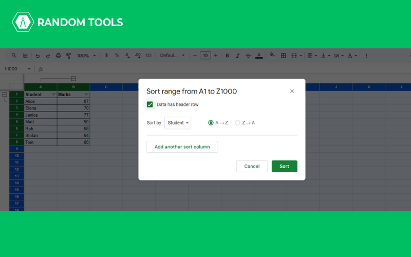
• Select the Sort Range, then click on Advanced Range Sorting Options. 

• Checkmark the Data has header now option. 
• Below that, you will Sort by option. Click the drop down beside that and select Region. 
• If you want to add another sorting option, click on Add another sort column. 
• Select from the drop down menu, and continue doing the same as per your requirement. You can also sort the data alphabetically (A-Z) or (Z-A).
• Click on Sort. 

How to Make a Table in Google Sheet – With Colors and Indicator Arrows

If you are using your table for inputting financial data, it is always advisable to use indicators to determine the percentage changes. Here’s how you can do it –

• Highlight the column where you want to add the indicator. 
• Go to Format and select Custom Number Format. 

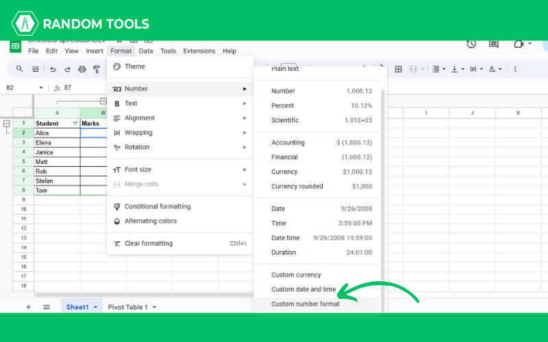
• Enter the custom numbers as follows – 0.00%▲; 0.00%▼; 0.00%

• The custom number will show the figures depending on whether the percentage is negative or positive. 

How to Delete Table Columns and Row in Google Sheets?

To delete the table all you need to do is clear formatting. All the colors, indicators, header color, etc, will be gone. Here’s how to do it –

• Select all.
• Go to Format and select Clear Formatting.
• 
• It’s Done!!

Conclusion

Now that you know how to make a table in Google Sheets, you must also understand creating a table along with formatting it correctly (as per your need) can help you get a better result. In addition, tables help you segregate your data, making the table look appealing. You can choose any of the methods as per your need, and of course, you can always customize the formatting. Now, if you want to learn Google Sheets basic, don’t forget to check the blog!