How to Freeze a Row in Google Sheets in 2023?

You must have thought at time – How to Freeze a Row in Google Sheets? It is quite understandable that it takes a good amount of scrolling to work with huge datasets, and losing sight of the cells you’re observing. The headers disappear when you scroll down, and the row disappears when you navigate to the right. Fortunately, with a few clicks, you can quickly freeze rows or columns in Google Sheets so that the important data is always visible. Thus, it is important to know how to freeze a row in Google Sheets!

In this tutorial, you will discover three distinct methods for freezing rows or columns in Google Sheets – 

• Drag-and-drop
• View menu
• Right-click menu. 

You will also learn how to use all three techniques to freeze several rows or columns.

How to Freeze a Row in Google Sheets?

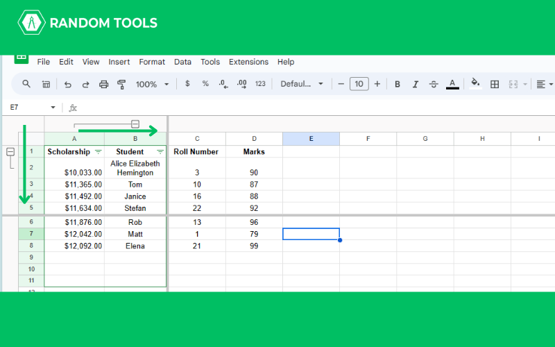
The easiest way to freeze rows in Google Sheets is the drag-and-drop method. Here’s how to do it –

• Go to the empty square, which is the point of intersection of row and column headers. (you’ll find the image below.)
• Click on the bottom line of the square and drag it until you want to freeze the row. 
• Now, drag the outline below the point you want to freeze. 
• To repeat the first column, repeat step one, grab the left-hand line of the corner cell, and drag it just beyond the column you want to freeze.
• The first row and column will always be visible, no matter how far down you have scrolled. 

How to Freeze a Row in Google Sheets – View Menu

This is another method to view the row in Google Sheets. Follow the steps to learn –

• Go to View>Freeze>Choose from the options available.

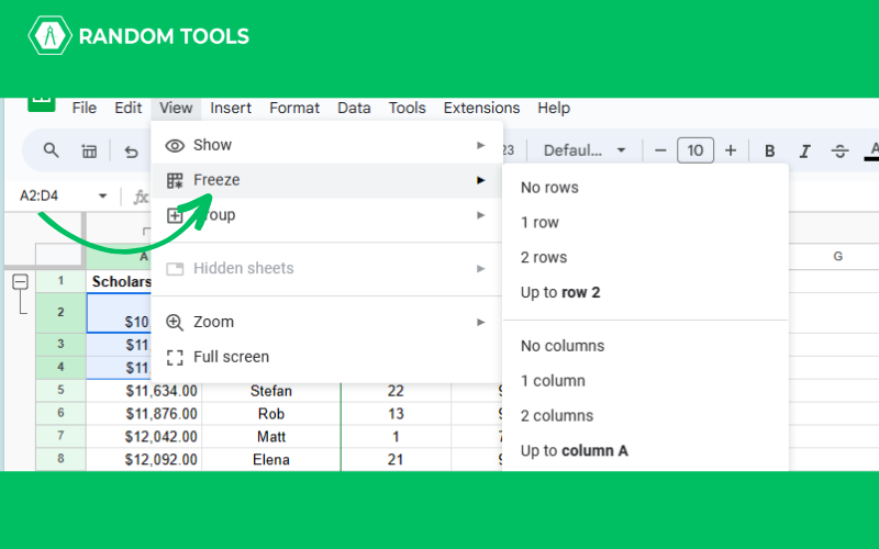
• One row is for the top row, and 2 row is to freeze the top two. 

How to Freeze a Row in Google Sheets – Right-Click Menu

Right-click menu is another method of freezing the rows. Here’s how you can do it –

• Click the row you want to freeze. 
• Right-click on the row number to view the menu option. 

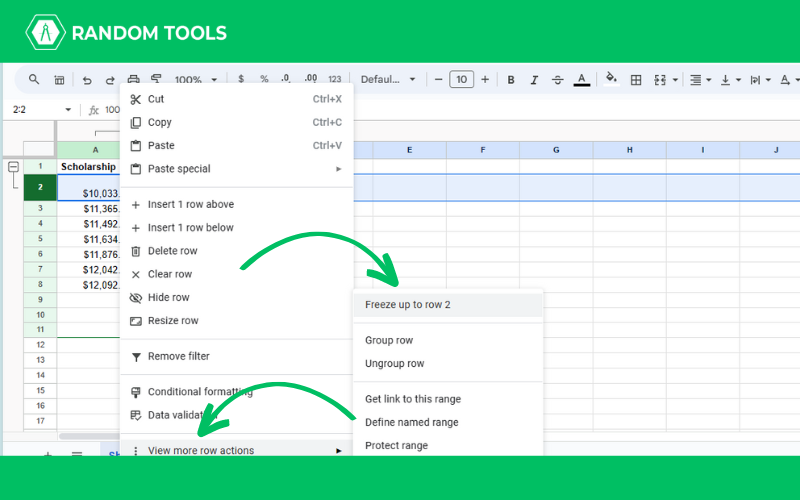
• Go to More Row Actions>Freeze up to row 2. 

You can also similarly freeze your columns. However, instead of selecting the rows, you have to choose the columns, then right-click and select the More Column Options.

How to Freeze a Row in Google Sheets – Multiple Row

You can freeze multiple rows simultaneously in Google Sheets using all three methods mentioned above. Here’s how all three ways look like –

Drag and Drop Shortcut

Drag and drop shortcut method is one of the easiest ways to freeze multiple rows. Here’s how you can do it –

• Go to the empty square, which is the point of intersection of row and column headers. 
• Click on the bottom line of the square, and drag it until you want to freeze the row, say four rows. 
• Now, drag the outline below the point you want to freeze. 
• The first rows will always be visible, no matter how far down you have scrolled. 

This way, it can also freeze the columns section. Repeat step one: Grab the left-hand line of the corner cell and drag it just beyond the column you want to freeze.

View Menu

You can freeze several cells by using the View method. Here’s how you can do it –

• Select the rows you want to freeze.
• Go to View>Freeze>Freeze up to row (X).

• Using the same method, you can freeze the columns as well. 

Right-Click Menu

Here’s how you can freeze multiple rows using the right-click menu –

• Select the row you want to freeze. 
• Right-click on the row.
• Click on View More Row Actions>Freeze up to row X(the number of rows you want to freeze). 

• You can use the same method to freeze the column. 

Conclusion

In Google Sheets, freezing rows or columns is simple and helpful. It can be challenging to keep an eye on the cells you want to examine when utilizing enormous datasets, and you have to scroll back and forth continuously. The top row or column can be frozen to ensure the headers are always visible.

Now that you know how to freeze a row in Google Sheets, you can use the right-click menu, the ‘View’ menu, or the drag-and-drop shortcut. This way, you can see not only the rows but also the columns. Want to learn more about such cool hacks? Visit Google Sheet Basics!